Geographic Interoperability Model

A geographic target looks like one object — "the New York market" — but it is handled as a chain of distinct objects, each a lossy or lossless transform of the last. Conflating them is the root cause of most "the numbers don't match" disputes between buying, execution, and measurement.

The canonical pipeline

Every arrow is a conversion documented elsewhere in this knowledge base, and every arrow can change the geography. The model exists so that each object has a name, a schema, and a provenance record — and so a claim like "we targeted the polygon" can be checked against what was actually executed.

The six geographies

Requested

The buyer's ask in their own vocabulary: a DMA id, a 3-mile radius, a named trade area. Often not a geometry at all — an identifier.

Source

The geometry actually supplied to represent the ask: a shapefile, a GeoJSON polygon, a point list. May already differ from the request.

Normalized

Source geometry validated and reprojected to EPSG:4326 GeoJSON: closed rings, correct winding, antimeridian split, holes respected.

Canonical H3

A set of H3 cells at a stated resolution under a stated containment rule. The interchange form all downstream conversions start from.

Executed

What a platform can actually run: point+radius circles, simplified polygons, or native geo IDs — an approximation of the H3 set.

Reported / attributed

The geography used for delivery reporting and outcome attribution — frequently coarser than what was executed.

Why provenance must survive conversion

Each hop should append to a ConversionRecord, never overwrite it. The minimum that must be recoverable at the end of the chain:

• the source CRS, vendor, and boundary vintage;
• the normalization actions taken (what was repaired);
• the H3 resolution and containment mode;
• the approximation mode used for execution (inner/outer/equal-area circle, polygon simplification tolerance, crosswalk vintage);
• which exclusions or targets were dropped because a platform could not express them.

Without this, you cannot answer the questions this knowledge base is organized around: what was requested, what was executed, and why do they differ?

A worked gap

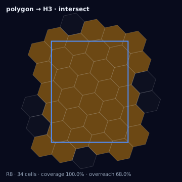
Suppose the request is a county (a partition unit), executed on a DSP that only accepts point+radius circles.

$\text{county polygon} \xrightarrow{\text{polyfill, R7, intersect}} \{h_1 \dots h_n\} \xrightarrow{\text{circumscribed}} \{(c_i, r_i)\}$

The intersect polyfill already overreaches at the county boundary; the circumscribed circles overreach again and overlap each other. The executed footprint is strictly larger than the requested county, and some ground is eligible under two circles at once. None of that is wrong — but it must be reported, via the quality metrics, not hidden behind the phrase "we targeted the county."

This page has no ts algorithm block of its own — the pipeline it narrates is coded page by page elsewhere in this knowledge base. As a short illustration, the same Requested → Canonical H3 → Executed steps with the Python bindings (h3-py v4):

import h3

# Requested -> Source -> Normalized: a county ring, already reprojected to
# EPSG:4326 as (lat, lng) pairs.
county_ring = [
    (40.70, -74.02), (40.70, -73.98),
    (40.74, -73.98), (40.74, -74.02),
    (40.70, -74.02),
]
county_shape = h3.LatLngPoly(county_ring)

# Normalized -> Canonical H3, at resolution 7.
# NOTE: h3-py's polygon_to_cells uses CENTER containment, like h3-js — the
# "intersect" rule this worked example uses is not a one-liner; it means
# classifying each candidate cell yourself (shapely intersection area
# against the source ring), exactly as the TS lib's polygonToH3 does.
canonical_cells = h3.polygon_to_cells(county_shape, res=7)

# Canonical H3 -> Executed: dissolve the cell set back into a polygon
# footprint (here, a stand-in for the circumscribed-circle executed
# geometry the worked example above actually uses).
executed_shape = h3.cells_to_h3shape(canonical_cells, tight=True)

The tested reference implementation in this knowledge base is the TypeScript in lib/, which implements the intersect and full containment rules explicitly rather than relying on h3-py's center-containment default.