Line And Corridor To H3

Purpose

Roads and device trajectories are one-dimensional (or effectively zero-width) geometries, which makes "convert to H3" ambiguous in a way polygons are not: a line has no interior to test cell centers against. This page distinguishes four legitimate conversions — intersection, sampling, buffered corridor, and network-distance corridor — and covers the trajectory-specific problems (noise, oscillation, dwell) that dominate in practice.

Source geometry and destination geometry

Source geometry is line_road (a static road-network segment or polyline) or trajectory (an ordered, timestamped sequence of device positions). Destination geometry is an h3_cell_set, or — for trajectories — an ordered H3 sequence with per-cell entry and exit timestamps, which is a materially richer object than an unordered cell set.

Exactness class

Approximate for all four variants below; a 1-dimensional line has zero width and therefore zero area, so any polygon-style containment fraction is either trivially zero or requires an explicit corridor width to become meaningful.

Containment rule and boundary behavior

Intersection

Include every H3 cell that the line geometry passes through, regardless of how short the intersection segment is. Cheapest and most common; corresponds to intersect-mode polygon containment applied to a zero-width geometry.

Sampling

Interpolate points along the line at a fixed step (e.g. every 25 m) and take the H3 cell of each sampled point. Cheaper to compute for very long lines but can skip cells the line passes through between samples if step size exceeds cell diameter.

Buffered corridor

Buffer the line by a stated half-width into a polygon, then polyfill that polygon under any of the four polygon containment modes. Turns a width-less line into a genuine area-bearing corridor with a defensible coverage_ratio.

Network-distance corridor

Include cells within a stated network-travel-distance (drive time or drive distance along the road graph) of the line, not Euclidean distance. Matches real accessibility catchments but requires a routable network graph, not just geometry.

For trajectories specifically, the output is not just a cell set but an ordered sequence: consecutive positions map to consecutive H3 cells (with repeats where the device stays in one cell), each annotated with entry timestamp, exit timestamp, and derived dwell time. Direction of travel is recoverable from the sequence order and should be preserved rather than collapsing the trajectory into a set before it is needed.

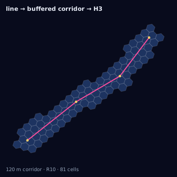
Resolution behavior

Intersection and sampling both produce thinner, more line-like cell sets at higher resolution and thicker, more blob-like sets at lower resolution, since a coarse cell straddling the line drags in area on both sides. Buffered-corridor coverage_ratio behaves like any polygon polyfill: it tightens toward the true corridor area as resolution increases. For trajectories, resolution also controls dwell-time granularity — at a resolution where consecutive pings fall in the same cell, dwell time is computed correctly as the span between entry and exit; at a resolution finer than the noise floor of the position data, a stationary device can appear to hop between adjacent cells purely from GPS jitter (see boundary-oscillation, below), fragmenting what should be one dwell event into many.

Units and CRS

EPSG:4326 for geometry; corridor buffer widths and network distances in meters; timestamps in UTC with explicit timezone handling for any day-part or dwell analysis performed downstream. Network-distance corridors require the routing graph's own distance units (often already meters) to be reconciled with the buffer width's units before comparison.

Algorithm

import { polygonToH3 } from "@/lib/h3/polyfill";
import { latLngToCell } from "h3-js";

// Intersection: cells the line touches at all
const intersected = polygonToH3(lineAsZeroWidthGeometry, {
  resolution: 9,
  mode: "intersect",
});

// Buffered corridor: give the line width, then polyfill normally
const corridor = polygonToH3(bufferLine(roadSegment, 100 /* m half-width */), {
  resolution: 9,
  mode: "intersect",
});

// Trajectory: ordered cell sequence with dwell
function trajectoryToCellSequence(pings, resolution) {
  const seq = pings.map((p) => ({
    cell: latLngToCell(p.lat, p.lng, resolution),
    t: p.timestamp,
  }));
  return collapseConsecutiveDuplicates(seq); // merges repeats into entry/exit/dwell
}

The same conversion with the Python bindings (h3-py v4):

import h3
from shapely.geometry import LineString, Point
from shapely.ops import transform
import pyproj

def buffer_corridor(line_lat_lng, half_width_m):
    # Buffer the line (in an azimuthal-equidistant frame centered on its
    # midpoint) into a corridor polygon, then polyfill it like any
    # arbitrary polygon.
    lats, lngs = zip(*line_lat_lng)
    mid_lat, mid_lng = sum(lats) / len(lats), sum(lngs) / len(lngs)
    aeqd = pyproj.CRS.from_proj4(f"+proj=aeqd +lat_0={mid_lat} +lon_0={mid_lng} +units=m")
    to_aeqd = pyproj.Transformer.from_crs("EPSG:4326", aeqd, always_xy=True).transform
    to_wgs84 = pyproj.Transformer.from_crs(aeqd, "EPSG:4326", always_xy=True).transform
    line_m = transform(to_aeqd, LineString([(lng, lat) for lat, lng in line_lat_lng]))
    corridor_m = line_m.buffer(half_width_m)
    corridor_deg = transform(to_wgs84, corridor_m)
    return [(lat, lng) for lng, lat in corridor_deg.exterior.coords]

def corridor_to_h3(line_lat_lng, half_width_m, res):
    ring = buffer_corridor(line_lat_lng, half_width_m)
    return h3.polygon_to_cells(h3.LatLngPoly(ring), res)  # center containment;
    # for intersect/full/threshold, classify candidates with shapely area
    # overlap exactly as on the arbitrary-polygon page.

# Ordered sequence for a trajectory, with grid_path/grid_distance available
# to interpolate or measure between non-adjacent cells in the sequence.
def trajectory_to_cell_sequence(pings, res):
    seq = [(h3.latlng_to_cell(p["lat"], p["lng"], res), p["t"]) for p in pings]
    # h3.grid_distance(a, b) reports hop count between two cells in the
    # sequence; h3.grid_path(a, b) fills in the cells presumed traversed
    # between two non-adjacent samples (e.g. a coarse sampling step).
    return collapse_consecutive_duplicates(seq)

The tested reference implementation for this conversion is the TypeScript in lib/; the Python above mirrors its buffer-then-polyfill and sequence-collapsing logic with core h3-py calls.

Parameters

Resolution, conversion variant (intersection, sampling, buffered corridor, network-distance corridor), corridor half-width or network distance, sampling step (sampling variant only), and — for trajectories — a smoothing window applied before cell assignment.

Outputs

For static lines: an h3_cell_set, optionally with coverage_ratio against a buffered reference corridor. For trajectories: an ordered list of {cell_id, entry_ts, exit_ts, dwell_seconds} records, one per contiguous occupancy of a cell, plus a derived direction-of-travel field between consecutive distinct cells.

Quality metrics

For buffered corridors: standard coverage_ratio, overreach_ratio, jaccard against the buffer polygon. For trajectories: cell-hop rate (hops per minute) as a proxy for noise — an implausibly high hop rate for a device's stated speed indicates boundary oscillation rather than genuine movement — and dwell-event count before and after smoothing, to quantify how much fragmentation smoothing removed.

Edge cases

GPS noise is the dominant real-world problem: consumer-grade GPS has a typical accuracy radius of 5-15 meters in open sky and 20-50+ meters in urban canyons, which is frequently larger than a res-10 or res-11 cell, so a stationary device's raw pings can scatter across several neighboring cells even with zero actual movement. Boundary oscillation compounds this specifically near a cell edge: a device whose true position sits within noise-distance of a cell boundary can flip between two cells ping to ping, manufacturing false dwell events and false direction changes; the standard mitigation is trajectory smoothing (a moving average or a map-matching step against the road network) applied before cell assignment, not after — smoothing the cell sequence itself cannot undo damage already done by assigning noisy points independently. Device-trajectory-exposure is a privacy and governance edge case, not a purely geometric one: an ordered, timestamped cell sequence at fine resolution is a de-anonymization vector for identifying home and work locations, and any pipeline producing this output should apply the resolution floors and aggregation minimums described in privacy and minimum aggregation before the sequence leaves a controlled environment.

Assumptions and limitations

This conversion assumes the caller has decided which of the four variants answers their actual question before running it — "does this campaign touch this road" (intersection), "what's the footprint of a 200m buffer around this corridor" (buffered corridor), or "what did this device do" (trajectory) are different questions with different correct answers, and none substitutes for another. Network-distance corridors additionally assume a maintained, routable road graph is available; where one is not, a buffered corridor with a conservative width is the honest fallback, not a silent substitute presented as network-aware.