H3 To Inscribed Circle

Purpose

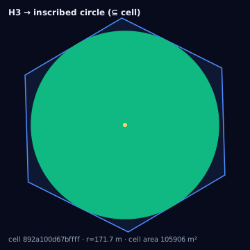
Many execution surfaces — mobile SDKs, DOOH proof-of-play radii, legacy DSPs — accept only a point and a radius, never a polygon. The inscribed circle is the point-radius approximation of an H3 cell that never claims ground the cell does not contain: it is the correct choice whenever the requirement is "do not target outside this cell," including mutually exclusive treatment/control cells in an experiment.

Source geometry and destination geometry

Source is an h3_cell_set, one circle computed per cell. Destination is point_radius: a center latitude/longitude and a radius in meters, one pair per input cell.

Definition

Center is the H3 cell center (cellToLatLng). Radius is the minimum geodesic distance from that center to any point on the cell's true boundary — not the nearest vertex.

Robust algorithm

Each of the cell's edges is a great-circle arc between two vertices, not a straight line in lat/lng space. The algorithm densifies every edge with DEFAULT_EDGE_SAMPLES = 64 evenly spaced great-circle (slerp) samples, computes the haversine distance from the center to every sample, and takes the minimum. A relative SAFETY_MARGIN = 1e-4 shrink is then applied to that minimum so the guarantee holds between the finite samples, not only at them — the true continuous minimum could fall slightly closer to center than any single sampled point, and the margin is sized to dominate the observed sub-1e-5 inter-sample error by an order of magnitude.

function inscribedRadius(cell):
    center = cellCenter(cell)
    boundary = cellBoundary(cell)          # great-circle arcs, vertex list
    samples = densifyGreatCircle(boundary, perEdge=64)
    minDist = +infinity
    for p in samples:
        d = haversineDistance(center, p)
        if d < minDist: minDist = d
    return minDist * (1 - 1e-4)            # SAFETY_MARGIN shrink

import { inscribedCircle } from "@/lib/h3/circles";

const approx = inscribedCircle(cell);
// approx.center: [lat, lng]
// approx.radiusMeters: minimum center->boundary distance, margin-shrunk
// approx.cellAreaM2, approx.circleAreaM2, approx.isPentagon

The same conversion with the Python bindings (h3-py v4):

import math
import h3

DEFAULT_EDGE_SAMPLES = 64
SAFETY_MARGIN = 1e-4

def _to_unit_vector(lat: float, lng: float):
    lat_r, lng_r = math.radians(lat), math.radians(lng)
    return (
        math.cos(lat_r) * math.cos(lng_r),
        math.cos(lat_r) * math.sin(lng_r),
        math.sin(lat_r),
    )

def _to_latlng(v):
    x, y, z = v
    return (math.degrees(math.asin(z)), math.degrees(math.atan2(y, x)))

def _slerp(a, b, t: float):
    # Spherical linear interpolation between two unit vectors; this is the
    # great-circle equivalent of a lerp, and what "densify with great-circle
    # (slerp) samples" means concretely — h3-py has no built-in densify call.
    dot = max(-1.0, min(1.0, sum(ai * bi for ai, bi in zip(a, b))))
    theta = math.acos(dot)
    if theta == 0:
        return a
    sin_theta = math.sin(theta)
    wa = math.sin((1 - t) * theta) / sin_theta
    wb = math.sin(t * theta) / sin_theta
    return tuple(wa * ai + wb * bi for ai, bi in zip(a, b))

def densify_edge_geodesic(a, b, samples: int = DEFAULT_EDGE_SAMPLES):
    va, vb = _to_unit_vector(*a), _to_unit_vector(*b)
    return [_to_latlng(_slerp(va, vb, i / samples)) for i in range(samples + 1)]

def inscribed_radius_m(cell: str) -> float:
    center = h3.cell_to_latlng(cell)
    boundary = h3.cell_to_boundary(cell)  # vertices only — NOT the full boundary
    n = len(boundary)
    min_dist = float("inf")
    for i in range(n):
        a, b = boundary[i], boundary[(i + 1) % n]
        for sample in densify_edge_geodesic(a, b):
            d = h3.great_circle_distance(center, sample, unit="m")
            if d < min_dist:
                min_dist = d
    return min_dist * (1 - SAFETY_MARGIN)  # shrink so the guarantee holds between samples

h3-py does not ship an inscribedCircle helper or a densify function — this reproduces the algorithm with core calls: cell_to_boundary for the vertex list, a great-circle (slerp) densify per edge, and great_circle_distance for each sample-to-center distance, taking the minimum across all densified samples and shrinking it by the same 1e-4 safety margin. Do not shortcut this to "minimum distance to a vertex" — that silently produces a circle too large to guarantee ⊆ cell, exactly as the danger callout above describes. The tested reference implementation is the TypeScript in lib/.

Containment guarantee

Every point of the inscribed disk lies inside the true H3 cell: inscribed disk ⊆ cell. This holds under the spherical model used throughout (haversine distance, cellArea on the same model) and within the 1e-4 safety margin against the finite-sample approximation of the boundary. It is the only circle construction in this section whose guarantee runs in this direction.

Resolution behavior

Radius scales with cell edge length, which shrinks roughly by sqrt(7) ≈ 2.65× per resolution step. Finer resolutions give proportionally smaller inscribed circles and proportionally smaller absolute uncovered corner area, but the relative underreach (uncovered area as a fraction of the cell) is resolution-invariant for regular hexagons — it is a function of cell shape, not cell size.

Units and CRS

Center and boundary coordinates are [lat, lng] (h3-js native order), EPSG:4326. Distances are spherical (haversine) meters on R_MEAN = 6,371,008.8 m, the same sphere cellArea uses, so radius and area figures are mutually consistent — not ellipsoidal (WGS84) survey distances.

Quality metrics

underreach_ratio

area(cell − inscribed disk) / area(cell). Always greater than zero for a hexagon; this is the uncovered-corner cost, not a defect.

uncovered_area

area(cell − inscribed disk) in absolute m², useful when comparing across mixed resolutions where the ratio alone hides magnitude.

For a perfectly regular hexagon the radius ratio inscribed/circumscribed is exactly $\cos(30°) \approx 0.866$ (apothem over circumradius) — real H3 cells are only approximately regular, so measured ratios cluster near but not exactly at this value, and pentagons and distorted cells sit further from it. The area comparison that matters for underreach_ratio is disk area against cell area, not disk against disk:

$\frac{\text{inscribed disk area}}{\text{cell area}} = \frac{\pi r_{in}^2}{\text{cell area}} = \frac{\pi \cos^2(30°)}{3\sqrt{3}/2} \approx 0.907$

for a regular hexagon — the inscribed disk covers about 90.7% of the cell, leaving underreach_ratio ≈ 0.093: roughly 9% of a regular hexagon's area, concentrated in its six corners, sits outside the inscribed disk. That 9% is the structural cost of the ⊆ guarantee, not a rounding error, and it is what makes the inscribed circle unsuitable whenever "complete coverage" is the actual requirement.

Edge cases

Pentagons have five, shorter, less regular edges; their inscribed radius is smaller relative to cell area than a hexagon's, so the underreach ratio is measurably worse at the 12 pentagon cells per resolution — flag them (isPentagon on the result) rather than silently averaging them into a fleet-wide radius estimate. Cells whose boundary crosses an icosahedron face seam are handled correctly by the distance-to-boundary algorithm (it makes no planarity assumption), but any downstream code that assumes a "typical" hexagon shape for these cells will be wrong. Antimeridian-crossing cells need longitude unwrapped before any lat/lng-based bounding logic runs; the haversine distance calculation itself is unaffected because it works in 3-D angle terms, not planar longitude differences.

Assumptions and limitations

Two neighboring inscribed circles never overlap with each other in the sense that matters for experiment isolation — no ground is double-covered — but they also do not tile the cell layer: uncovered gaps exist at every cell's corners and are not claimed by any neighbor's circle either. That makes the inscribed circle the right choice for mutually exclusive treatment cells and the wrong choice for "complete coverage" requirements, which belong on the circumscribed circle page instead.